
Starting a few years before the 2020 census, the bureau began discussing methodologies for improving ‘disclosure avoidance’. To be honest, we were highly skeptical of how this would play out, especially since the published methodology discussions were obtuse, reading like the specifications for a Rube Goldberg machine. We were convinced that the Census folks were so immersed in the purity of the theoretical that they neglected to test their techniques on real data until after the census was administered. It is only recently that results of tests on the 2010 census have become available.
When the PL-94 redistricting release came out, we dove into the data immediately. Within half an hour, our internal Teams chat was jammed with maps, tables, mean-spirited GIFs, and more than a few words momma told us never to use. In one of our first blog posts, we characterized the most absurd cases as ghost, mermaid, baseball team, and Lord of the Flies census blocks.
While the industry was doing cartwheels and shouting from the rooftops, AGS was busy manning the ice-water bucket brigade. The initial reaction of our competitors ranged from crickets to outright mocking, but undeterred, we pressed on. While others simply published the data as it was and hoped their users wouldn’t notice, we spent a couple of months in the basement doing some restoration work on the data.
We were also busy building our geographic correspondence tables so that we could accurately migrate data between the 2010 and 2020 block geographies, which was critical since most were still using the old boundaries.
With a good restoration of the 2020 data and flexible tools for integrating data from sources using both old and new geographies, we were able to properly integrate the PL-94 data into our data – and any of our users can request both the out-of-the-box and revised versions of our 2020 base data.
The DHC release of the census has created additional challenges, especially at the block level, where the DA methods very much tend to ‘clump’ similar groups together. In order to preserve the totals of two-dimensional matrices (e.g. age by sex), the methods tend to disallow small numbers and therefore push counts away from those values (usually the 2-4 range for any cell). Even at the block group level, the effects of the DA modifications can be clearly seen. For example, we can look at the male to female ratio of 21-year-olds in Ventura County, California block groups. When the 2020 data is compared to 2010’s, we can see a clear increase in the scatter of the values.
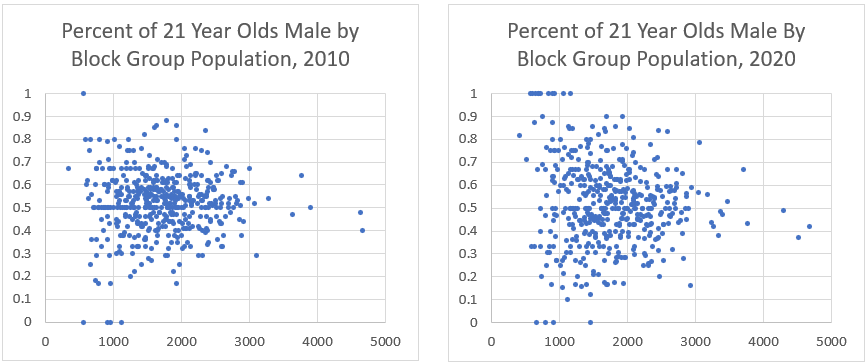
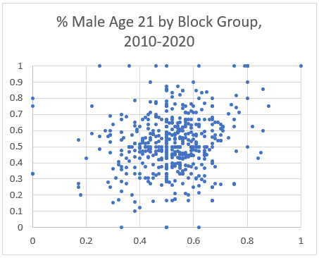
Further, if we look at a scatter plot between 2010 and 2020 percent male, we see that many have shifted dramatically. We would expect to see a clear pattern along the line from (0,0) to (1,1) but instead see a very ‘boxy’ pattern, with many points shifting from strongly dominant male to dominant female and vice versa.
So, what does this mean? First, if you use the data ‘out of the box’, any statistical models which rely on detailed age, sex, or race distributions will be seriously impacted. Second, any work done which relies on these as a starting or control point for time series analysis will result in a highly error prone projection results.
It is for these reasons that we believe that the census data must be approached with a carefully thought out and well executed plan. Using external data sources in conjunction with matrix balancing techniques is required to minimize the inconsistencies. This will provide a stable base moving forward over the decade.

Recent Comments