Many data sources which appear to be national coverage at a specific geography level will often have missing records. There are a wide variety of methods which can be used to ‘infill’ missing records from the simplistic (assign it the average value or a geographically scoped average value) to complex (create a model for each missing variable).
By way of example, as part of our reconstruction of our ‘quality of life’ series, we worked with some excellent data at the Census tract level produced by the Centers for Disease Control that look at the incidence of chronic health conditions and a range of risk factors thought to influence them. As we almost always do, we threw the data up on a map long before we read the documentation – realizing that we needed the 2010 tract roster not the 2020 one. There were scattered missing records, as we would usually expect that cover areas with zero or near zero population. These rarely pose a problem, since zero records usually stay that way, and near-zero can be easily assigned values from adjacent areas, usually by using an inverse distance weighting. What these maps showed, however, was a much more substantial problem: an entire state of missing data. And not a small one either.
So how did we handle the issue?
Fortunately, disease incidence and the associated risk factors are very strongly related to demographic characteristics, so we used our own analytics dataset – Demographic Dimensions – to fill in the missing data.
The Dimensions database can be used to create a demographic signature for any location which we have discussed elsewhere for use in site selection models. We began by a simple assignment of the 2010 census tract data to 2020 block groups. We broke the block groups into three parts –
- The target block groups, which had no health data
- The selection pool of block groups, which have health data and a minimum population
- Exclusion block groups, which had data, but not enough population
Since demographics are predictors of these variables, the goal for each target was to find, from the selection pool, the most demographically similar block groups from which we could ‘borrow’ data.
The data borrowing technique can be refined, especially if the between demographics and the target variable is not particularly strong, by:
- Imposing a geographic filter, whereby we only consider block groups in the selection pool if they are within a specified distance of the target block group.
- Using the median or average of the values found for the n-closest signatures.
In this particular case, the relationships are so strong that we simply found the most similar block group from the selection pool and ‘borrowed’ its data.
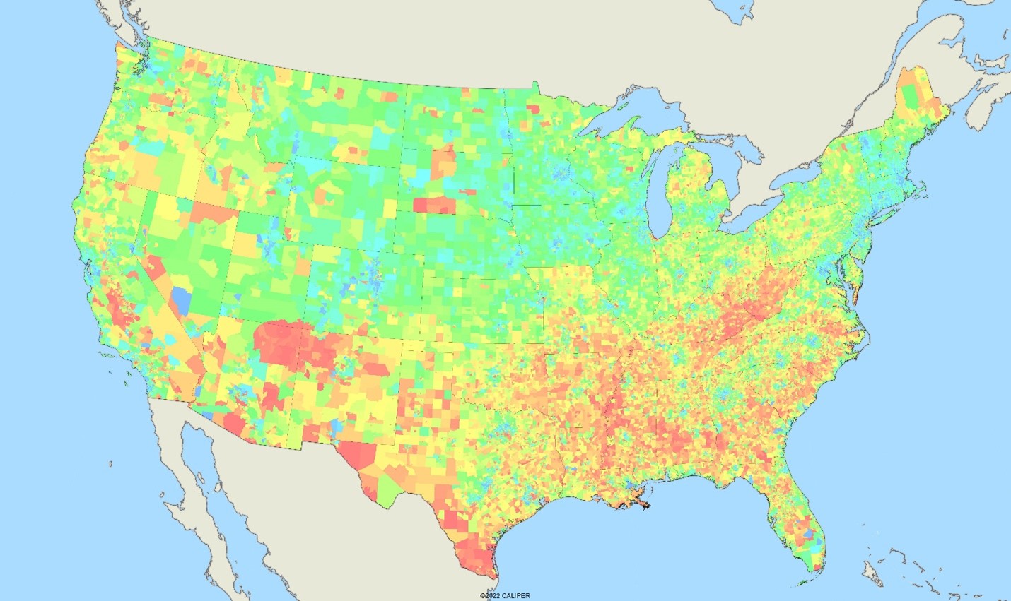
The results can be validated in a couple of simple ways. With an entire state missing the first approach is to find similar data at the state level and check the goodness of fit. In this case, we thought it might be interesting to show the raw results – without cheating by reading the documentation, can you tell what state actually had no data?
The map here is the percentage of adults who say they are in “poor or fair” general health – which ranges from about 8% (blue) to over 40% (red):
As always, our data nerds are always eager to help with questions ranging from where you can find it to what can (and should) you do with it and everything in between. Sometimes, the data just needs a good esthetician…. we have one.
Oh, and the missing state? New Jersey.