
Income is one of the most commonly used variables in demographic analysis. Whether you’re evaluating a retail trade area, planning a new development, or sizing up a potential customer base, income is often treated as the go-to measure of purchasing power. But in reality, income is usually just a surrogate. What we really want to understand is demand—and demand is often much more specific than simply asking how much money people make.
That’s one reason AGS offers far more than a single household income variable. Depending on the application, you may need the income of homeowners ages 35–54, household income for households with two or more vehicles, or income for families with children. Different products appeal to different consumers, and a one-size-fits-all income measure often misses the mark.
One of the most common questions we receive is whether our income estimates are adjusted for the cost of living. At first glance, that seems like a simple request. If an area’s cost of living is 20% above average, shouldn’t its income be discounted by the same amount?
The challenge is that “cost of living” is surprisingly difficult to define.
Most cost-of-living indexes compare the prices of common goods such as gasoline or groceries, often at the state or metropolitan level. The Consumer Price Index (CPI), for example, measures the cost of a standardized basket of goods. While useful for many economic purposes, these measures have limitations when applied to local market analysis.
Housing costs can vary dramatically between neighboring communities—or even neighborhoods within the same city. Tax burdens differ substantially from one jurisdiction to another. And perhaps most importantly, spending patterns aren’t the same for every household. A retired couple, a young family, and a high-income executive all spend their money very differently. Averaging these households together often washes out the very differences analysts are trying to measure.
Instead, AGS approaches the problem from the household level. Using our Synthetic Household model, we estimate expenditures for individual households, accounting for local differences in housing costs while also reflecting regional spending patterns. Rather than relying solely on broad averages, we build estimates from the bottom up.
That allows us to focus on two measures that often matter more than total income:
- Disposable income: Household income after federal, state, and local taxes, along with Social Security and Medicare deductions.
- Discretionary income: What’s left after taxes and essential expenses such as housing, groceries, and utilities.
For many consumer products, discretionary income is a much better indicator of purchasing power than total income alone.
The differences can be dramatic. Consider four affluent counties:
| County | Average Household Income | Average Disposable Income | Average Discretionary Income |
| Westchester, NY | $211,807 | $122,472 | $76,850 |
| New York (Manhattan), NY | $217,351 | $114,977 | $79,583 |
| Fairfax, VA | $204,240 | $142,118 | $91,298 |
| Williamson, TN | $197,451 | $139,641 | $90,194 |
Although Manhattan has the highest average household income, households in Fairfax County and Williamson County actually have substantially more discretionary income available to spend after taxes and essential expenses. Even Westchester, despite a lower average income than Manhattan, leaves households with more money available after accounting for local living costs.
The accompanying map illustrates another way to think about this concept. It shows the relative burden of non-discretionary expenses across the country. Coastal metropolitan areas, where housing costs are typically highest, stand out with above-average and high expense levels. Much of the Midwest and South, by contrast, generally shows lower non-discretionary costs, meaning households often retain more spending power than income figures alone would suggest.
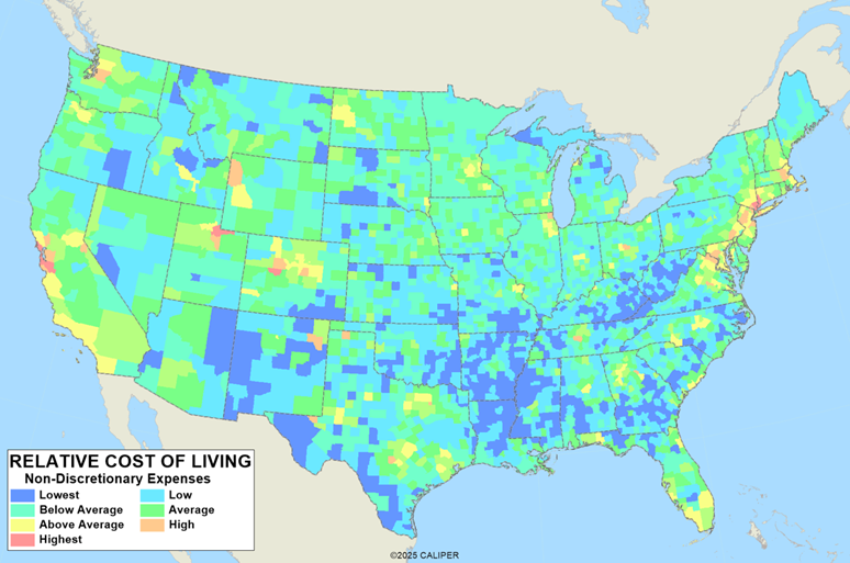
For retailers, banks, restaurants, and countless other businesses, this distinction matters. A high-income trade area isn’t always the market with the greatest purchasing power. In many cases, a nearby community with lower incomes—but significantly lower taxes and housing costs—may actually have more discretionary income available for consumer spending.
Income will always remain an important demographic measure. But when your goal is to understand demand rather than simply reporting earnings, disposable and discretionary income provides a clearer picture of consumer behavior. They require a bit more explanation than a simple income figure—but they also lead to better decisions. And ultimately, that’s the measure that matters most.