Spatial Autocorrelation

In recent years, data science and analytics have emerged from the backroom to become mission critical for many companies. Linear regression and its many variants are foundational to that effort and its core assumptions are commonly known and understood. The basic linear model takes the form –

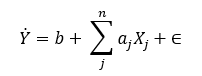
The predictors of Y, variables through are assumed to be independent of each other – so for example, we would not attempt to estimate a model where the independent variables are known to be closely related. Autocorrelation is present when the independent variables are related, and if significant, has a major effect on both the efficiency and bias of the model.

With geospatial analysis, the problem is generally known as ‘spatial autocorrelation’. In 1970, Waldo Tobler formulated his first law of geography: “Everything is related to everything else, but near things are more related than distant things.” When we are using spatial units, such as census block groups, as the observation unit in regression, it must be understood that autocorrelation will by definition exist in both the dependent and independent variables. Spatial autocorrelation is both the reason why spatial analytics works in the first place and quite frequently, why it doesn’t.

Site location analytics relies on the existence of spatial autocorrelation. Without it, there would be no concentration of potential customers and any location would be just as good as any other. Two great examples below were taken from the excellent study notes of Manuel Gimond, available at https://mgimond.github.io/Spatial/index.html:

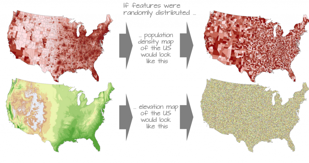
Spatial autocorrelation has been described as both a nuisance and a feature of geospatial analytics since it both complicates model performance and interpretation while at the same time being the only reason why we would use spatial models in the first place. It is the high level of spatial autocorrelation which makes the interpolation of elevation possible in the first place.

There are some measures of spatial autocorrelation which are readily available in mapping and statistical packages, including Moran’s I (which can be computed locally or globally) or Geary’s contiguity ratio.

From a practical perspective, those engaged in spatial analytics need to be aware of issues that can arise when using geographically aggregated data (such as ZIP codes or census blocks) for the purposes of predictive modeling:

• Avoid at all costs using autocorrelated predictor variables. For example, you usually shouldn’t use both per capita income and median years of education as predictors in a model. One way to add demographics to spatial prediction models is to use the AGS Demographic Dimensions modeling set, which are free of autocorrelation and standardized. Note that they can be spatially autocorrelated, which is a feature not a bug in most cases.
• For any model, make sure you map the residuals, that is, the difference between the predicted and observed values. Residual analysis is often overlooked by analysts, especially if the models seem to fit well in the first place. Very rarely do we find analysts mapping the residuals looking for spatial autocorrelation in them. Ideally, a model which predicts something like market share by census block group should have little spatial autocorrelation in the residuals. If present, a spatial regression model may be necessary in order to account for distance decay or agglomeration effects, or additional potential explanatory variables should be sought.

Interested in exploring spatial analysis further? We recommend the book Geospatial Analysis, authored by Michael de Smith, Michael Goodchild, and Paul Longley (2018) which is an excellent resource for both data scientists and programmers.