The AGS synthetic household model was introduced with the completely new Household Finances database earlier this year. Over the past few months, we have been busy expanding the demographic content of the household model in order to provide a base for the new Consumer Expenditure dataset which will be released in November. Part of that expansion includes the ability to look at disposable income as the base for consumer spending, rather than total household income.
Confusingly, economists refer to disposable income as that which remains after federal, state, and in a few cases, local income taxes are levied. Discretionary income is defined as disposable income less essential expenditures – shelter and food.
The disposable income model relies upon the synthetic household base variables of age of householder, tenure, household size, number of vehicles available, and of course, household income. At the household level, it is much more feasible to reasonably estimate the tax burden by using state specific marginal tax rates, standard deduction amounts, and likely filing status.
The result is the ability to remove what are primarily state level differences in the disposable income available to similar households in different cities – a key step towards creating a discretionary income model.
The two maps below display, using the same classification, the sometimes radical difference between average block group income and disposable income:
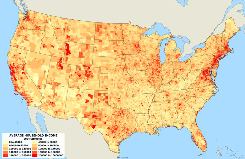
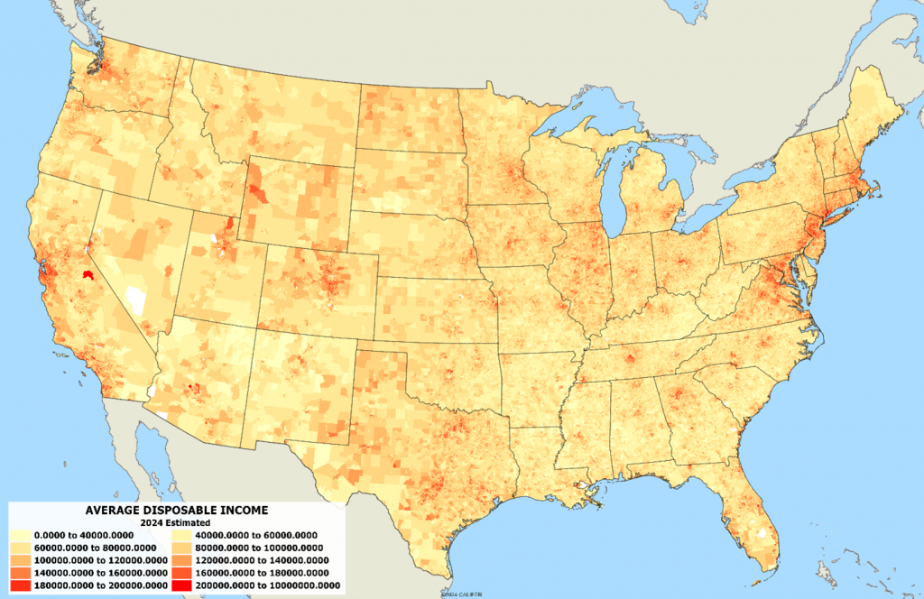
Clearly urban areas tend to have higher income levels, but there are some rural areas (western Wyoming and northern Colorado in particular) where incomes are high. It is when we display the average tax burden that the benefits of using disposable rather than total income for retail modeling is apparent:
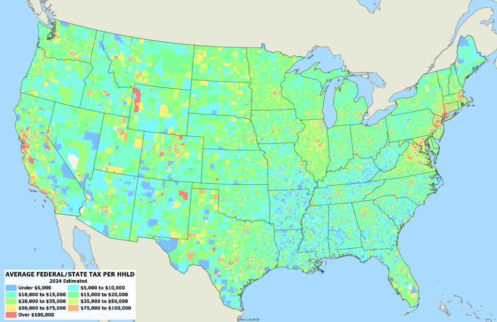
Obviously, areas with higher incomes have higher average taxation, but the net result is to substantially level the playing field. Note the clear delineation of Illinois on the map, given that the state income tax is substantially higher than its neighbors.